Consider a closed, nonconvex figure in the plane. What is its largest convex subset? Though this does seem like a well founded question, the largest convex subset turns out to be challenging to compute.
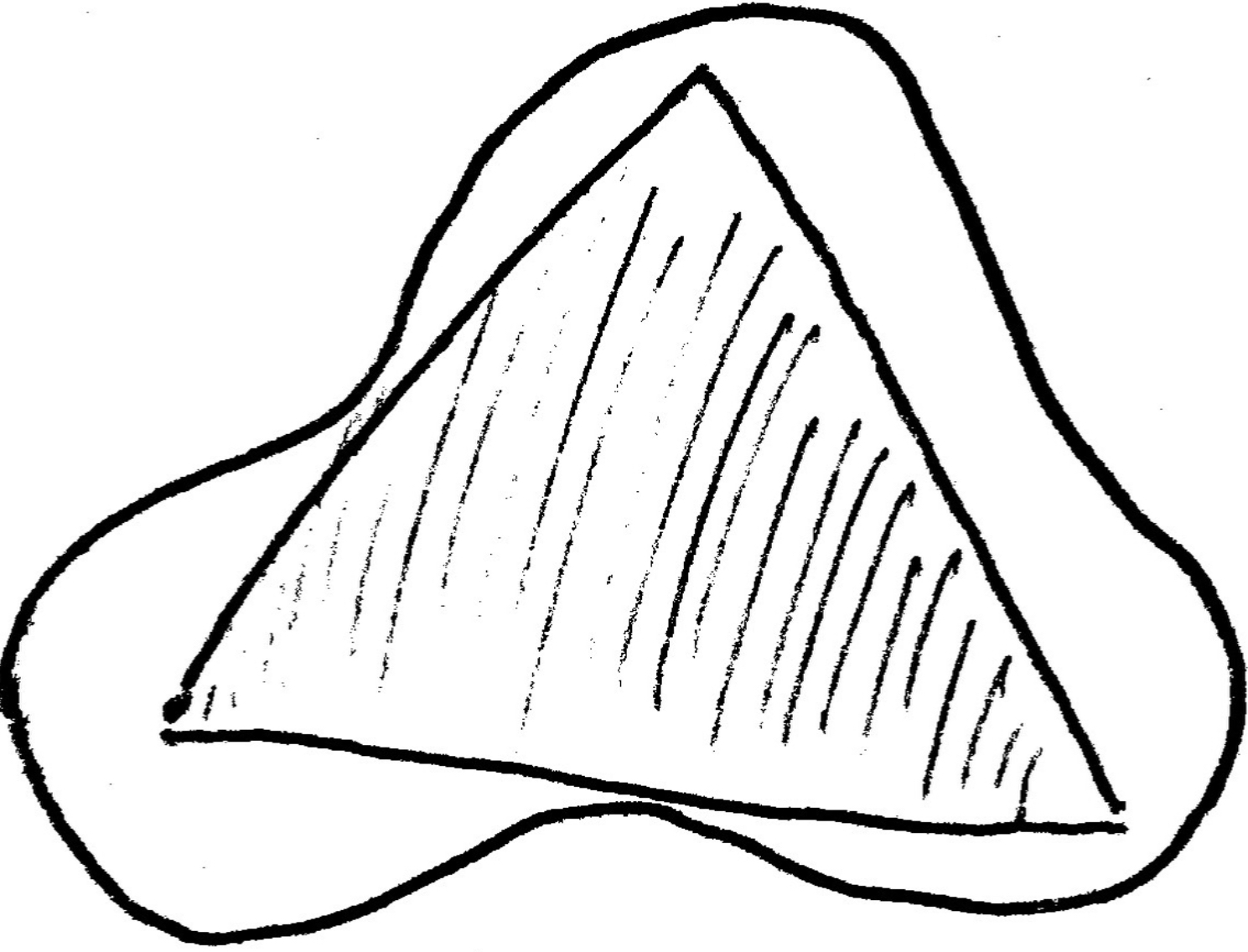
Figure 1 illustrates the question at hand. The amoeba shape is the nonconvex set in question, and the shaded triangle is a guess at the largest convex subset. Don’t look to closely though, it’s easy to pick out ways in which the triangular estimation can be improved. For instance, the bottom and left sides should be flush with the amoeba, and the right side of the triangle should also be pushed further until it’s flush (Figure 2).
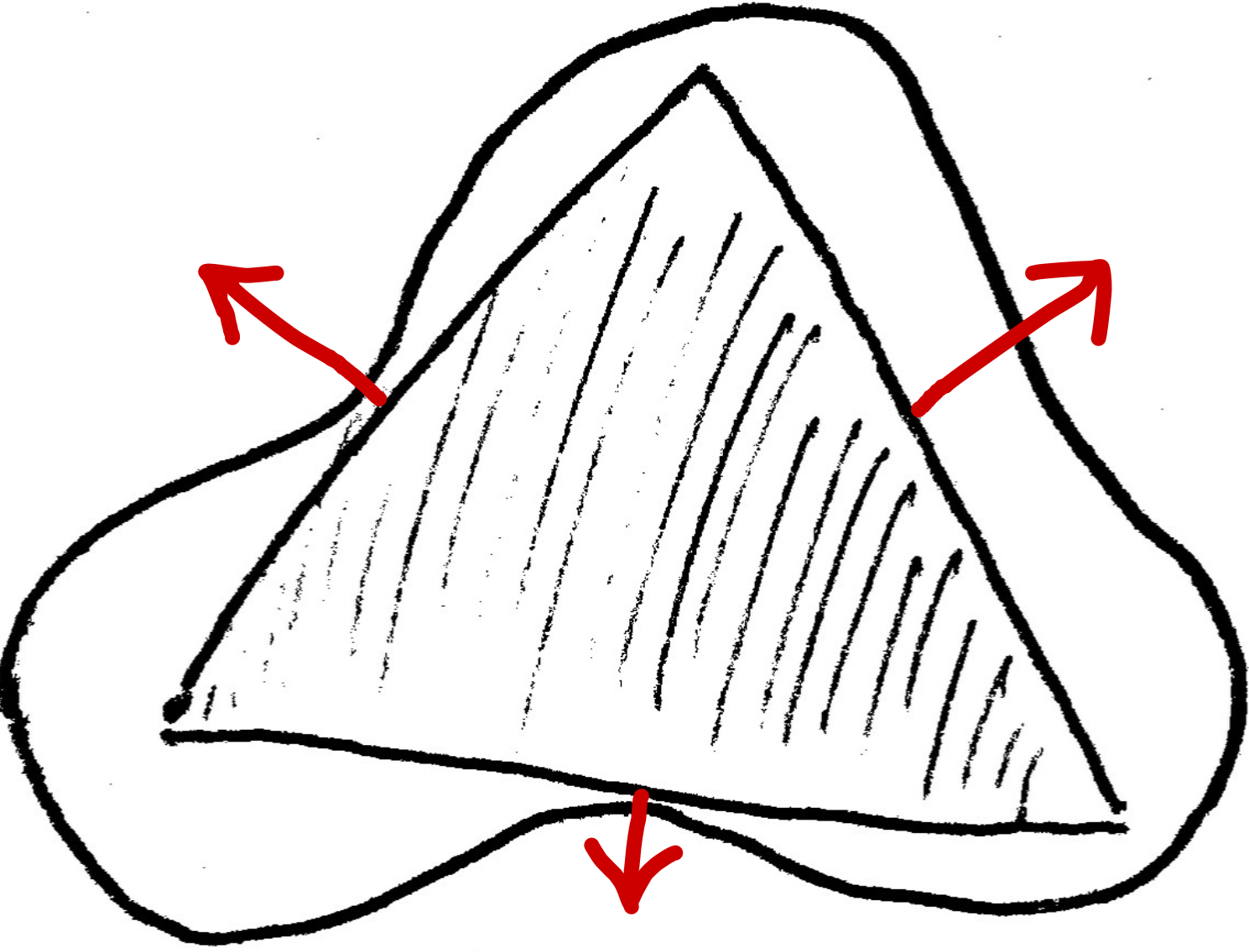
Of course, we also need to consider tradeoffs of curvature. Would the northwest
side of the triangle capture more area if it curved outwards like one half of
an oval? We’d better formalize the problem.
We’re optimizing over a collection, a set of sets. If we call the nonconvex set \(S\), the collection of interest here is \[C=\{\ T\subset\mathbb{R}^2 \mid \mathcal{[}T\subset S\mathcal{]}\ ;\ \mathcal{[}\lambda x+(1-\lambda) y\in T\ \ \forall\ \ \lambda\in [0, 1],\ (x,y)\in T\mathcal{]}\ \}\] The expression is a lot to parse, so I’ve written the two constraints with \(\mathcal{[}\)calligraphic brackets\(\mathcal{]}\) around them, and with a semicolon separating them. The first constraint is that \(T\) must be a subset of \(S\), and the second is that \(T\) must be convex. In plain english, \(C\) is just the set of all subsets of \(S\) that are convex.
What we’re missing, in order to have an well-formulated optimization problem, is an objective. How can we express the area of one of the subsets? For a convex set in the plane, we can compute its area with a double integral. For instance, for our sets \(T\in C\)
\[\textbf{area}(T)=\iint_Tdx\;\!dy\]
Let’s calculate a few very simple double integrals to get a feel for what’s going on. There are two informal ways to think about double integrals that I’ve seen. The first is approaching the computation as two, sequential integrals – one in \(x\) in the other in \(y\):
\[\int_{y_0}^{y_f}\int_{x_0}^{x_f}dx\;\!dy\ .\]
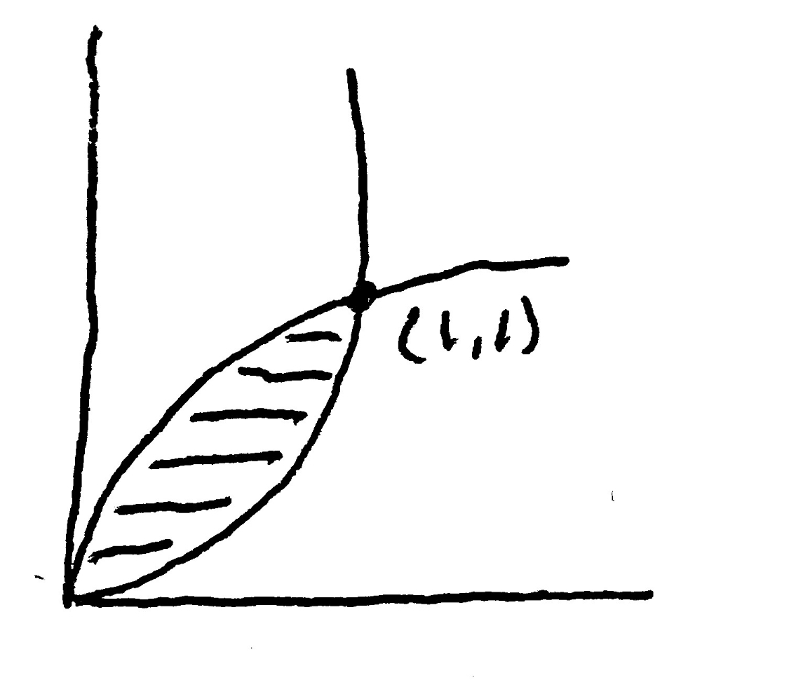
A simple example is computing the area enclosed by \(y=\sqrt{x}\) and \(y=x^2\). Let the inner integrals (integrals plural, since we have an \(x\)-integral for each term of the \(y\)-integral) be over \(dx\). The inner integrals will vary in their bounds as a function of \(y\), and the outer integral is bounded by the lower and upper extent of the figure in the \(y\)-dimension.
\[\int_{y=0}^{y=1}\int_{x=y^2}^{x=\sqrt{y}}dx\;\!dy=\frac{2}{3}y^{3/2}-\frac{1}{3}y^3\bigg\vert_0^1=\frac{1}{3}\]
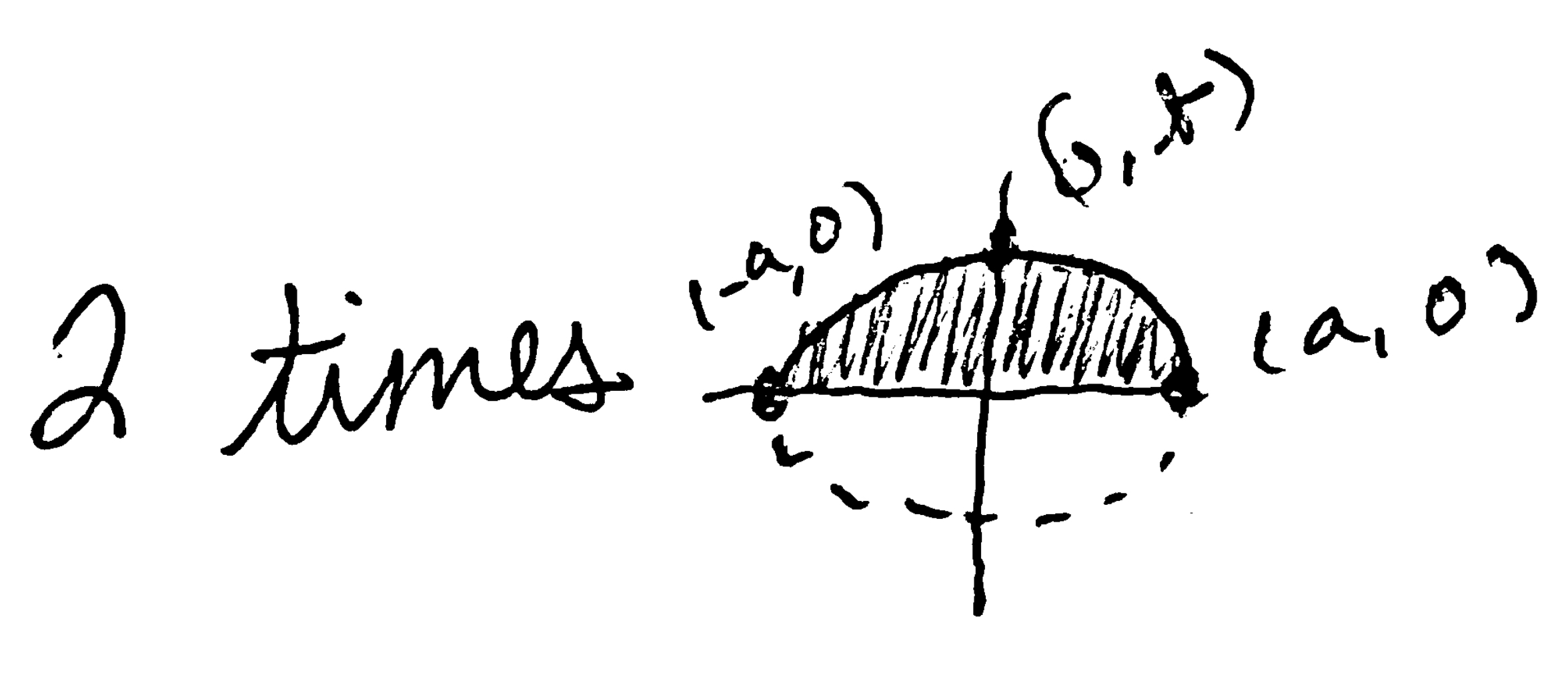
[7/16/23 ] If you wanted to compute the area of an ellipse, one approach would be to isolate the top half of the ellipse, compute the area between it and the \(x\)-axis, and then double the result to get the total area. The procedure would look something like this: start with an ellipse \(E\)
\[E(a',b',r)=\left\{(x,y)\in\mathbb{R}^2\ \bigg\vert\ \left(\frac{x}{a'}\right)^2+\left(\frac{y}{b'}\right)^2=r^2\right\}\ .\]
Note that we can simplify the expression by defining \(a=a'r\) and \(b=b'r\).
\[\implies E(a,b)=\left\{(x,y)\in\mathbb{R}^2\ \bigg\vert\ \left(\frac{x}{a}\right)^2+\left(\frac{y}{b}\right)^2=1\right\}\ .\]
Working with the constraint, we isolate \(x\), integrate, then double to get the area:
\[y=b\sqrt{1-\left(\frac{x}{a}\right)^2}\]
\[\implies\textbf{area}(\:\!E(a,b)\:\!)=2\int_{-a}^{a}b\sqrt{1-\left(\frac{x}{a}\right)^2}\ dx\ .\]
Consider the substitution \(x/a=sin(\theta)\implies dx=a\cos(\theta)d\theta\), giving
\[2ab\int_{\pi}^{0}\cos^2(\theta)\ d\theta\ .\]
The integral of \(\cos^2(\theta)\) can itself be solved by a substitution, \(\cos^2(\theta)=\frac{1+\cos(2\theta)}{2}\):
\[2ab\int_{\pi}^{0}\cos^2(\theta)\ d\theta = ab\left[\int_{\pi}^{0}\ d\theta+\int_{\pi}^{0}\cos(2\theta)\ d\theta\right]\]
\[=ab\left[\arcsin(x/a)+\frac{1}{2}\sin(2\arcsin(x/a))\right]\bigg\vert_{-a}^{a}\ .\]
Though at this point we could simply plug in the bounds, here’s one last trick. To simplify the second term, notice that
\[\sin(2x)=2\sin x\cos x\implies\sin(2\arcsin(x/a))=2(x/a)\cos\left(\arcsin(x/a)\right)\ .\]
In our integral, we’re left to evaluate \(\cos(\arcsin(x/a))\). Arcsine is the function which takes a value of sine (i.e. in the interval \([-1, 1]\)) and maps it to the first angle (increasing, starting from \(-\pi/2\)) that yields it as the angle’s sine value. In our case, \(\arcsin(x/a)\) is wrapped in \(\cos()\), meaning that our output is the associated cosine value of the sine value we originally passed as input to the arcsine, such that the pairing lies on the unit circle.
To further understand the exact pairing of sine-value \(x\)-coordinates to cosine-value \(y\)-coordinates, we can pass the entire interval \([-1, 1]\) through arcsine and observe that it produces the interval \([-\frac{\pi}{2},\frac{\pi}{2}]\). As the argument of cosine varies from \(-\frac{\pi}{2}\) to \(\frac{\pi}{2}\), the output of cosine varies from \(0\) to \(1\) and back to \(0\). Having observered that the input-output pairings of \(\cos(\arcsin(x/a))\) form the upper half of the circle, we can conclude that
\[\cos(\arcsin(x/a))=\sqrt{1-\left(\frac{x}{a}\right)^2}\ .\]